Blog
Computer Vision and Remote Sensing: Agricultural Information in the 21st Century
July 23, 2020
By Ernesto Brau At CIBO, we are focused on providing actionable information and insights regarding farmland, and we use many different sources of data to do so. Some of this data is available from public sources. Some we derive from our proprietary modeling technology. And other data comes to us from tens of thousands of miles in the air, via satellites soaring around the earth. Some of the celestial data we use in our innovative app is from the National Oceanic and Atmospheric Administration’s satellites, which provide storm images dating back to 1960. Recently launched imaging satellites, such as the Landsat and Sentinel constellations, also give us access to a vast amount of information. This all raises the question: what exactly are we extracting from these remotely sensed images? The answers are surprisingly varied and point to a new era in agriculture, where global information systems inform local decisions. 
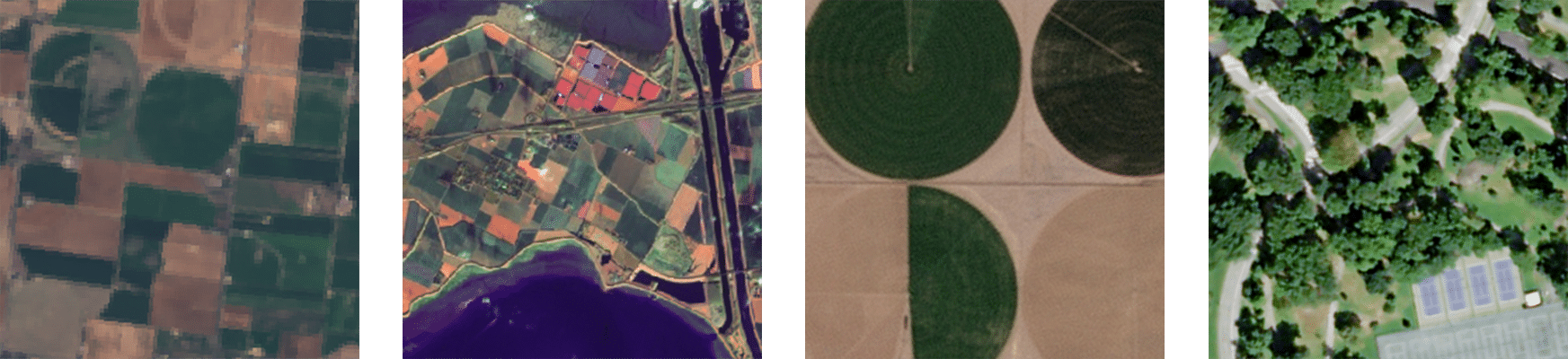
Figure 1: Examples of satellite imagery. From left to right, images from the Landsat 8, Sentinel-2, RapidEye, and SkySat satellites.
Land Cover Classification
Knowing the land cover of a region is extremely useful for many agricultural applications, such as determining the acres planted of different crops. Estimating land cover from images is called land cover classification, and it is a very important task in remote sensing. The most well-known instance of this is the Cropland Data Layer (CDL), a product provided yearly by the United States Geological Survey (USGS). CDL is produced using a decision tree algorithm to classify pixels into one of 256 classes, including both crop (e.g., corn and soybean) and non-crop (e.g., forest and water) cover types. Figure 2 shows an example of the CDL output. Naturally, the usefulness of CDL depends on its accuracy, which varies drastically by class: for very common crops like corn and soybean, the accuracy is over 90%. For other crops, however, it can dip well below 50%.

Figure 2: An example of CDL classification on several parcels in Kansas. The different colors represent different types of land use — e.g., yellow and brown
Land cover classification has been approached in a wide range of other ways, with varying degrees of success. These efforts include: low-level segmentation strategies (e.g., using edge and circle detection); machine learning models such as decision tree classifiers (like CDL) and support vector machines; and even deep learning, using convolutional neural networks to classify small patches of images. However, we have yet to see an attempt that incorporates the latest image segmentation techniques, such as fully convolutional nets (FCNs), the U-Net model, and their successors. At CIBO, we believe new land classification methods can provide improved speed and accuracy of CDL-like results.
Crop Phenology
Crop phenology is the observation and study of plant life cycles. Just as we capture important milestones in our lives, agronomists record critical time points in the life of a plant or crop. These milestones vary from crop to crop: a corn farmer is concerned about when tasseling will occur, while a cotton farmer wonders whether squares are setting.
Remotely sensed images, particularly from satellites, can be used to study the phenology of planted crops at a large scale. This is done by temporally tracking the vegetation index (VI) of a crop, a measurement designed to give high values for growing vegetation. The most widely used VI is the normalized difference vegetation index (NDVI), which is defined as 
where red and NIR are the pixel values of the red and near-infrared channels, respectively. Since vegetation typically has a low reflection in the red and a strong reflection in the near-infrared, NDVI has a value of near one for pixels containing vegetation. The VI evolution through time can be modeled using several functions. See Figure 3 for an illustration of the VI values for a field, as well as a fitted model curve.

Figure 3: The VI phenology curve. On the left, the NDVI values of a corn field over a period of one year. On the right, a typical "double-sigmoid" curve detailing the same NDVI observations.
Because VI curves have a strong correlation with the green vegetation stages of growth, we can use these curves to estimate the timing of emergence and maturity of the crop. Additionally, characteristic differences in the VI curves of different crops can be exploited by a machine learning algorithm to improve land cover classification results (as described in the previous section).
Remote Assessment of Field Stability
Agricultural fields do not usually have uniform performance across their geographic extent. In particular, some areas of a field can have highly variable performance from year to year, while others are very stable and will reliably produce high yield every season. Measuring the within-field performance stability is useful for many different reasons; for instance, it can help determine regions of a field that need to be managed differently, or where new equipment should be installed. Doing this at scale — that is, for large numbers of fields — is even more important.
As mentioned above, we can use VI as a proxy for vegetation, which itself is correlated with crop yield. By analyzing VI images of fields over multiple years, we can provide essential insights into field stability, such as determining which regions are stable over time and which ones are consistently high performing and low performing. Figure 4 illustrates this idea.

Figure 4: Field stability assessment over 10-year period. On the left, an image of a field in Nebraska. On the right, an image illustrating the different zones of the field: red indicates unstable performance while yellow, light green, and dark green indicate low, average, and high stable performance, respectively.
Field Irrigation Detection
Vegetation indices like NDVI (see above) can also help us determine whether an agricultural field has been irrigated. In particular, vegetation in fields that use pivot irrigation has a very distinctive appearance (see Figure 5). We can use machine learning and AI algorithms to distinguish VI images of irrigated and non-irrigated fields, and even to determine which parts of the field were irrigated. Indeed, from a computer vision perspective, this can be seen as an image segmentation problem, and there are dozens of ways to approach it, including modern AI techniques such as FCNs and U-Net. 
Figure 5: Example of irrigation detection. On the left, a satellite image of several fields that employ pivot irrigation. On the right, a segmentation of the left image where irrigated pixels are white and non-irrigated pixels are black.
Remote Detection of Standing Water
Accumulation of water in parts of a field can cause ponding, leading to crop damage and reduced yield. Detecting standing water regions in fields at a large scale is very useful and has many applications, such as land valuation and management practice assessment. There are several spectral indices that exhibit a strong response to water that are very helpful for this problem, such as the normalized difference water index (NDWI), which uses the following formula:

where Xgreen and Xnir are the values for the green and NIR channels, respectively. NDWI is designed to give high values for pixels contained in bodies of water, which makes it particularly useful to detect areas of standing water (see Figure 6). Although NDWI gives us clues as to where water tends to pond, there are still a number of challenges we need to overcome to solve this problem, such as dealing with regions of water that are smaller than an image pixel. We also need to examine what to do during the peak of the growing season, when canopy cover makes it impossible to see the ground from above.

Figure 6: NDWI image of a metropolitan area bordering the sea, encoded using a red-yellow-blue color palette, where red corresponds to low values and blue to high values.
Conclusion
The vast (and growing) amount of remotely sensed data, in particular satellite imagery, collected over the past few years creates an opportunity for new and widespread insights into agricultural practices and land use. To this end, CIBO is building tools that combine cutting-edge technology from computer vision and artificial intelligence applied to multiple remote sensing applications, such as land cover classification, phenology analysis, irrigation detection, and many others. As a result, CIBO will continue to provide the deepest, most data-rich insight into every parcel of land in the United States.
[1] All accuracies discussed are national accuracies for CDL in the year 2019. For FAQ concerning the CDL, see the CDL website.
About Ernesto Brau
Ernesto Brau is the Lead Computer Vision Scientist at CIBO, a science-driven software startup. Prior to CIBO, he worked on computer vision for AiBee Inc., Intel Corporation, and Hewlett-Packard Laboratories. He holds a Bachelor of Science in Computer Science from the Universidad de Sonora in Mexico, along with an MS and PhD in Computer Science from the University of Arizona.